Hidden Markov Model (HMM) Tutorial

This page will hopefully give you a good idea of what Hidden Markov Models (HMMs) are, along with an intuitive understanding of how they are used. They are related to Markov chains, but are used when the observations don't tell you exactly what state you are in. To fully explain things, we will first cover Markov chains, then we will introduce scenarios where HMMs must be used. There will also be a slightly more mathematical/algorithmic treatment, but I'll try to keep the intuituve understanding front and foremost.

Markov Chains §

Markov chains (and HMMs) are all about modelling sequences with discrete states. Given a sequence, we might want to know e.g. what is the most likely character to come next, or what is the probability of a goven sequence. Markov chains give us a way of answering this question. To give a concrete example, you can think of text as a sequence that a Markov chain can give us information about e.g. 'THE CAT SA'. What is the most likely next character? Another application is determining the total likelyhood of a sequence e.g. which is more likely: 'FRAGILE' or 'FRAMILE'?

Markov chains only work when the states are discrete. Text satisfies this property, since there are a finite number of characters in a sequence. If you have a continuous time series then Markov chains can't be used.

To define a Markov chain we need to specify an alphabet i.e. the possible states our sequence will have e.g. . For text this will be the letters A-Z and punctuation. For proteins this would be the 20 possible amino acids etc. We also need transition probabilities e.g. what is the probability of 'H' following 'T'? Finally we need the probability of characters on their own (the a priori probabilities) e.g. what is the probability of a random character being 'F'.

Once we have these things, we can calculate the probability of a sequence:

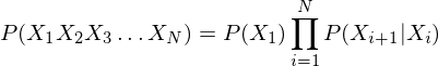
where is the probability of character given that was previous (this is the transition probability). The expression gives the probability of the sequence , assuming the sequence is a first order markov process i.e. each character only depends on the immediately preceding character. In general this is not true for text, a higher order model will perform better. Using a higher order model will require more transition states, and more training data to estimate the transition probabilities.

To train the transition probabilities for a markov chain you need lots of training data. For English text this will be many sentences. Given this training data we can count the number of times each character follows each other character, then get probabilities by dividing the counts by the number of occurrences. What can happen is that certain trainsitions will have a count of 0. If this transition occurs in testing, it will give a probability of 0 to the whole sequence, which is generally not wanted. To get around this psuedocounts are added. There are algorithms for determining what all the unseen transitions should be e.g. Kneser–Ney smoothing among many other algorithms.

Hidden Markov Models §

For Markov chains we had a state sequence e.g. characters and we always knew what the states were, i.e. there was no uncertainty. Imagine a scenario where instead of reading the characters from a page, we have a friend in a sound proof booth. He can read the characters out and we have to determine what characters he is saying by lip reading. In this case our states are the same characters as the markov chain case (characters on a page), but now we have an extra layer of uncertainty e.g. it looked like he said 'P', but 'P' looks alot like 'B', or maybe it was even 'T'. What's important is we can give the probability of a particular observation given that we are in a particular state.

When we speak about HMMs, we still have the transition probablities between states, but we also have observations (which are not states). Note that we never actually get to see the real states (the characters on the page) we only see the observations (our friend's mouth movements). One of the main uses of HMMs is to estimate the most likely state sequence given the observations i.e. what was written on the page given the sequence of observations. You can imagine the difficulty: if we know the previous state we can multiply the transition probability to the next state by the observation probability, but we don't know the previous state either! So we have to estimate them all at once. We will cover the algorithms for doing this below.

Another example where HMMs are used is in speech recognition. The states are phonemes i.e. a small number of basic sounds that can be produced. The observations are frames of audio which are represented using MFCCs. Given a sequence of MFCCs i.e. the audio, we want to know what the sequence of phonemes was. Once we have the phonemes we can work out words using a phoneme to word dictionary. Determining the probability of MFCC observations given the state is done using Gaussian Mixture Models (GMMs).

The extra layer of uncertainty i.e. not being able to look at the states, makes working with HMMs a little bit more complicated than working with markov chains. There are several algorithms for working with HMMs: for estimating the probability of a sequence of observations given a model the Forward algorithm is used. Given a sequence of observations and a model, to determine the most likely state sequence the Viterbi algorithm is used. Finally, given a lot of observation/state pairs the Baum-Welch algorithm is used to train a model.

A mathematical treatment §

The previous sections have been a bit hand wavey to try to convey an intuitive motivation for HMMs. If you want to implement them though, we need to get a little bit more rigorous. In the Markov chain, each state corresponds to an observable event, i.e. given an event we can say with 100% accuracy which state we are in. In the HMM, the observation is a probabilistic function of the state. A HMM is basically a Markov chain where the output observation is a random variable generated according to an output probabilistic function associated with each state. This means there is no longer a one-to-one correspondence between the observation sequence and the state sequence, so you cannot know for certain the state sequence for a given observation sequence.

A Hidden Markov Model is defined by:

• - An output observation alphabet. The observation symbols correspond to the physical output of the system being modeled. For speech recognition these would be the MFCCs.
• - A set of states representing the state space. is denoted as the state at time . For speech recognition these would be the phoneme labels, for text it would be the set of characters.
• - A transition probability matrix, where is the probability of taking a transition from state to state .
• - An output probability distribution, where is the probability of emitting symbol when in state .
• - An initial state distribution where

A complete specification of an HMM includes two parameters and , representing the total number of states and the size of the observation alphabet, the observation alphabet , and three sets of probability measures , , . A HMM is often denoted by , where . Given the definition above, three basic problems of interest must be addressed before HMMs can be applied to real-world applications:

1. The Evaluation Problem. Given a model and a sequence of observations , what is the probability that the model generates the observations, .


2. The Decoding Problem. Given a model and a sequence of observations , what is the most likely state sequence in the model that produces the observations.


3. The Learning Problem. Given a model and a sequence of observations , how can we adjust the model parameter to maximise the joint probability i.e. train the model to best characterise the states and observations.

Evaluating an HMM §

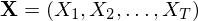
The aim of evaluating an HMM is to calculate the probability of the observation sequence , given the HMM . The steps involved in calculating are shown below. The algorithm is called the forward algorithm.

To calculate the likelyhood of a sequence of observations, you would expect that the underlying state sequence should also be known (since the probability of a given observation depends on the state). The forward algorithm gets around this by summing over all possible state sequences. A dynamic programming algorithm is used to do this efficiently.

You may wonder why we would want to know the probability of a sequence without knowing the underlying states? It gets used during training e.g. we want to find parameters for our HMM such that the probability of our training sequences is maximised. The Forward algorithm is used to determine the probability of a an observation sequence given a HMM.

• Step 1: Initialisation
  
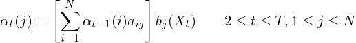
• Step 2: Induction
  
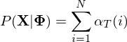
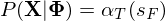
• Step 3: Termination
  
  If the HMM must end in a particular exit state (final state $s_F$) then,
  

Understanding the Forward Algorithm §

The forward algorithm can be understood to be working on a matrix of values. The values of represent the likelyhood of being in state i at time t given the observations up to time t. You can visualise the alpha values like this:

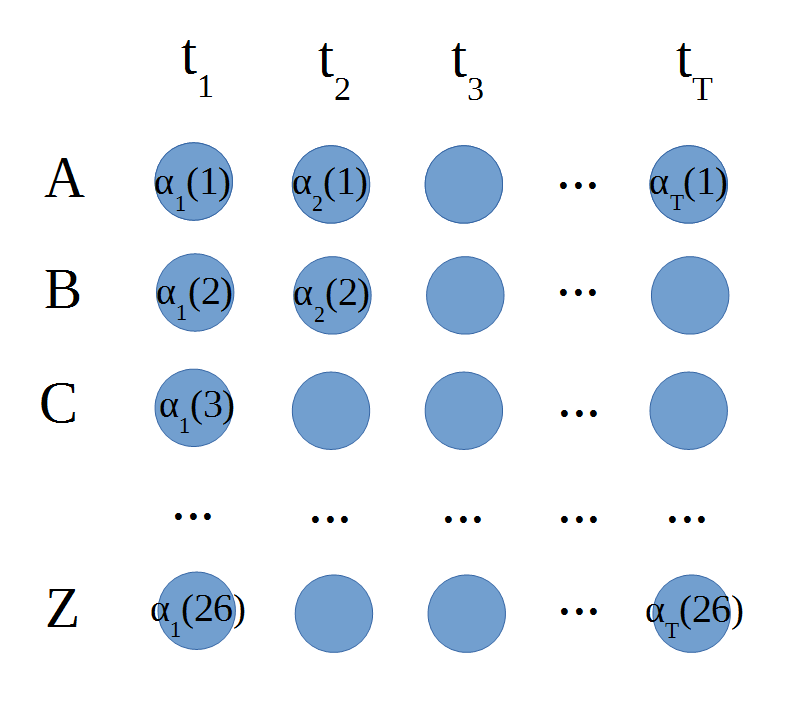
The blue circles are the values of alpha. is the top left circle etc. The initilisation step from the previous section fills the first column. Since there is no previous state, the probability of being in e.g. state 1 at time 1 is just the probability of starting in state 1 times the probability of emitting observation : i.e. . Once we have done that for all the states initialisation is complete.

The induction step takes into account the previous state as well. If we know the previous state is e.g. state 2, then the likelyhood of bein in state 4 in the current time step is i.e. the likelyhood of being in state 2 previously, times the transition probability of going from state 2 to state 4, times the probability of seeing observation in state 4. Of course, we don't know the previous state, so the forward algorithm just sums over all the previous states i.e. we marginalise over the state sequence.

Remember the job of the forward algorithm is to determine the likelyhood of a particular observation sequence, regardless of state sequence. To get the likelyhood of the sequence we just sum the final column of alpha values.

The Viterbi algorithm is almost identical to the forward algorithm, except it uses argmax instead of sum. This is because it wants to find the most likely previous state, instead of the total likelyhood. To find the best state sequence we backtrack through the latice, reading off the most likely previous states until we get back to the start.

Decoding an HMM §

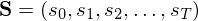
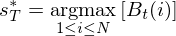
The aim of decoding an HMM is to determine the most likely state sequence given the observation sequence and the HMM . The steps involved in calculating are shown below. The algorithm is called the Viterbi algorithm.

The viterbi algorithm is very similar to the forward algorithm, except it uses argmax instead of summing over all possible sequences. This is necessary to enable us to pick the most likely sequence. It would seem like argmax is discarding a lot of information and should result in suboptimal results, but in practice it works well.

• Step 1: Initialisation
  
  
• Step 2: Induction
  
  
• Step 3: Termination
  
  
• Step 4: Backtracking
  
  

Estimating HMM Parameters §

Estimating the HMM parameters is the most difficult of the three problems, because there is no known analytical method that maximises the joint probability of the training data in a closed form. Instead, the problem can be solved by the iterative Baum-Welch algorithm, also known as the forward backward algorithm. The forward backward algorithm is a type of Expectation Maximisation algorithm algorithm.

The idea is to find values for such that the probability of the training observations (calculated using the forward algorithm) is maximised. We perturb the parameters until they can no longer be improved. I won't go into the details here, an outline is given below.

1. Initialisation. Choose an initial estimate .
2. E-step. Compute auxiliary function based on .
3. M-step. Compute according to the re-estimation equations on page 392 of Spoken Language Processing to maximise .
4. Iteration. Set , repeat from step 2 until convergence.

comments powered by Disqus