A Guide to Principal Component Analysis (PCA)

Introduction §

The definition of PCA uses eigenvectors and eigenvalues, concepts which can be rather confusing to those who don't already understand them. I will try to explain them here, but you may have to consult a few other tutorials/definitions to get a good feeling for what they really are. A good tutorial with pointers to more is here.

Let's start with the definition of eigenvector/eigenvalue (remember they come in pairs): An eigenvector is a property of a square matrix. Each square matrix has a set of eigenvectors, and if you change the matrix, it will usually change the eigenvectors. A 2 by 2 matrix has 2 eigenvectors and 2 eigenvalues, A 3 by 3 matix has 3 eigenvectors and 3 eigenvalues etc. Eigenvectors and Eigenvalues are just things we can calculate given a square matrix.

Pick an arbitrary 2 by 2 matrix, and call it A. If we choose an arbitrary point in 2-dimensional space, say 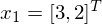, then we can use A to change the point .
e.g. if 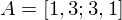, then the product is


So we can see the vector [3,2] gets sent to [9,11] when multiplied by the matrix A. The plot of and can be seen below:

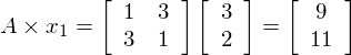
From the figure we see that A has stretched the vector x₁ (it's length went from 3.6 to 14.2) and it is also been rotated around the origin. This means that [3,2] is NOT an eigenvector of A, since its angle changed after multiplying it. What if we now multiply A by a new vector, x₂ = [1, 1].
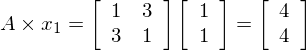
So we can see the vector [1,1] gets sent to [4,4] when multiplied by the matrix A. The plot of and can be seen below:

From the figure we see that A has stretched the vector x₂ (it's length went from 1.41 to 5.65) and it has NOT been rotated around the origin. This means that [1,1] IS AN eigenvector of A, since its angle didn't change after multiplying it. This is all an eigenvector is. It so happens that for a 2 by 2 matrix there are only 2 eigenvectors (up to scaling), for a 3 by 3 matrix 3 eigenvectors etc.

The eigenvalue is the amount the vector is scaled. In the example above, the eigenvalue for the eigenvector [1,1] is 4, since it was strtched by 4.

The Covariance Matrix §

The PCA algorithm is applied to the covariance matrix of a set of data, I will now explain why the eigenvalues and eigenvectors of a covariance matrix are important. I will use matlab code as psuedocode to explain it.

If we have a single dimension of zero mean unit variance data, and we wish to give it a specific variance, we must multiply it by the square root of the variance. e.g. to give 1000 data points a variance of 5,

X = sqrt(5) * randn(1000,1);
var(X) = 5.3175

In the above snippet we create a vector of 1000 random values with zero mean and variance of 1. We then multiply every point in the vector by sqrt(5), then measure the variance of the resulting vector. Our result is pretty close to 5, which means we were successful.

This can be extended to multivariate random data. In this case randn will return data with each dimension zero mean unit variance. If you were to plot it, it would form a spherical "ball" centered at zero. To give it a specific covariance, we multiply the data by the square root of the desired covariance matrix:

 X = randn(100000,3)*sqrtm([3,   1,  0.5; 1,   2,  -1; 0.5, -1, 1]);
 cov(X) =    
 2.9953    1.0046    0.4936
 1.0046    1.9885   -0.9931
 0.4936   -0.9931    0.9942

which is what we wanted. From this we can see that the covariance matrix (or at least the square root of it) is a transformation matrix that squishes our data around, sends some parts outwards, pulls some parts inwards and rotates some parts around a bit. Here we come to the definition of an eigenvector: it is a vector that, after being multiplied by the matrix, is only scaled (not rotated in any way). It so happens that the only points in our data that are scaled and not rotated when multiplied by the covariance matrix are those that lie in the principle directions of the distribution i.e. the axes of the multivariate gaussian. This means the eigenvectors are these axes, the eigenvalues happen to be the variance in the direction that corresponds to the eigenvector it is paired with.

PCA for decorrelation §

If we have a set of points such that some of the dimensions are correlated, we can use PCA to transform the data so that the dimensions are no longer correlated. This is achieved by multiplying the data by the matrix of eigenvectors, where each eigenvector is a column in the matrix.

data = randn(1000,2)*sqrtm([3, 1; 1, 3]);
covmatrix = cov(data);
[eigval,eigvec] = eig(covmatrix);
decorrelated = data*eigvec;    

The variable decorrelated now holds the decorrelated version of data.

PCA for whitening §

The point of whitening is to make all directions have unit variance. This is achieved by using the matrix of eigenvectors to decorrelate the data, followed by dividing by the eigenvalues to normalise the variance, then multiplying by the transpose of the eigenvectors again to undo the decorrelation. Undoing the decorrelation step means the data still looks like the original i.e. the correlations between dimensions still exist.

data = randn(1000,2)*sqrtm([3, 1; 1, 3]);
covmatrix = cov(data);
[eigval,eigvec] = eig(covmatrix);
decorrelated = data*eigvec;    
normalised = decorrelated./repmat(sqrt(diag(eigval)),size(data,1),1);
reconstructed = normalised*eigvec';

PCA for dimensionality reduction §

Dimensionality reduction is pretty easy, it is the same as PCA for decorrelation, except we don't multiply by the whole matrix of eigenvectors, only the columns with the highest eigenvalues.

data = <M by N matrix>
covmatrix = cov(data);
[eigval,eigvec] = eig(covmatrix);
[s,ind] = sort(diag(eigval));
reduced = data*eigvec(:,ind(1:K));    

reduced is now a K-dimensional matrix, where K < N. It can be used instead of data, it contains most of the variance in data, since the dimensions we dropped off were all the low variance dimensions.

comments powered by Disqus