Fitting a polynomial to a set of points

Interpolation can be defined as a method for estimating values that lie between two known values. Polynomial interpolation is the interpolation of a given data set by a polynomial, with the aim being to find a polynomial which goes exactly through the points. Polynomial interpolation usually means finding an order polynomial that fits points. Once the polynomial is found, it can be used to interpolate new, unseen data points.

To perfectly fit a polynomial to data points, an order polynomial is required. To restate slightly differently, any set of points can be modeled by a polynomial of order . It can be shown that such a polynomial exists and that there is only one polynomial that exactly fits those points. Considering that there is only one polynomial that fits a set of points, why would we be interested in knowing more than one algorithm for finding that polynomial? Each algorithm is used in its own niche areas.

The Vandermonde Matrix method §

This method is probably the easiest to understand, but also the least computationally efficient. We will do an example with the following numbers:

x	y
0	0
4	2
10	6
12	6.5

The Vandermonde method requires building the following matrices:

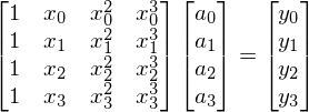
If we use our example points, we get the following:

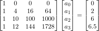
Our equation looks like this:

We can calculate the vector by inverting :

This can be solved very easily by e.g. Matlab. The result is:

so 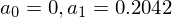etc. This gives us the coefficients for the interpolating polynomial. The main problem with this method is that matrix inversion is . The next two appoaches are .

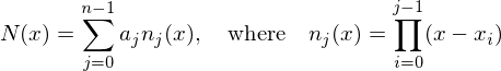
The Lagrange method §

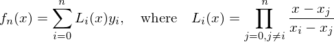
The Lagrange method was first published by Waring (1779), rediscovered by Euler in 1783, and published by Lagrange in 1795. The Lagrange method of interpolation is given by:

We will use the same points as in the previous example. We have 4 points, which means an order 3 polynomial will fit the data. This means will be our interpolating polynomial. So from the equation above,

With the Lagrange polymonials we can now find , our interpolating polynomial. The next equation combines equations for through to and the values of .

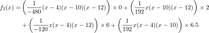
If we multiply everything out and combine terms, we are left with the following result:

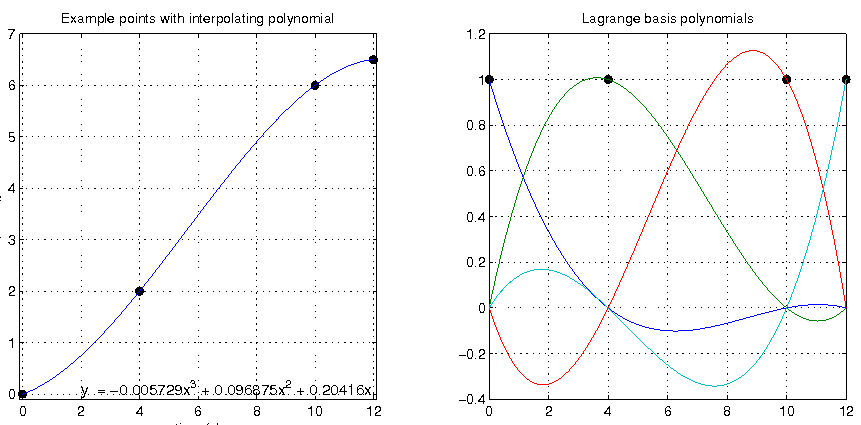
This is the same as the result we got for the Vandermonde method. We can plot this curve with the original points, see below. To understand how this method works, it is necessary to understand the basis polynomials, . Each basis polynomial is constructed so that it goes through 0 for all of the values except the , for which it has the value 1. Each basis polynomial is then scaled by , so the basis polynomials go through for the point in they correspond to, and zero for all the other points. These polynomials are then added up to get the final result.

The Newton method §

The Newton Method of polynomial interpolation relies on 'divided differences'. It is similar to the Lagrange method in that it is a linear combination of basis functions, but in this case the basis functions are the Newton polynomials. Given n points,

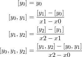
In the above equation, is defined as , with the square brackets being the notation for divided differences. This means the newton polynomial can be written as

The divided differences are defined recursively as follows:

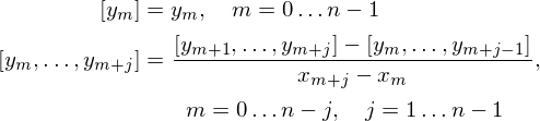
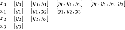
The easiest way to see all this working is using a quick example. We will use the same points as those used above. The first step is to caculate the divided differences to . Using the recursive definition we saw above, we can find

We can lay these values out in a table like the following:

which after solving becomes

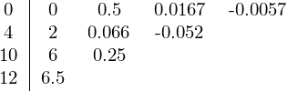
The values of that we need can be read from the top line: 0, 0.5, 0.0167, -0.0057. We now use the first equation we introduced in this section to find .

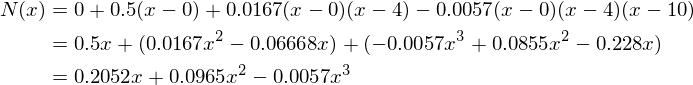
So once again we end up with the same interpolating polynomial.

Neville's Algorithm §

If an interpolated value is required, but the actual interpolation polynomial coefficients are not, Nevilles algorithm can be used. Neville's algorithm is based on the Newton method, and is a recursive algorithm defined as follows (given n+1 (x,y) pairs):

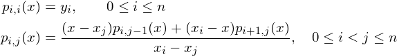
With the aim being to find the value of . The C implementation is provided below.

/************************************************
#### IMPORTANT -- contents of y are destroyed
Inputs: x   -   x values, array[0..N-1].
        y   -   y values, array[0..N-1].
        n   -   number of x or y values
        t   -   interpolation point
Return: the interpolated value of y at x=t
************************************************/
double neville_algo(double *x, double *y, int n, double t){
   int m = 0;
   int i = 0;
   for(m = 1; m < n; m++){
      for(i = 0; i < n-m; i++){
         y[i] = ((t-x[i+m])*y[i]+(x[i]-t)*y[i+1])/(x[i]-x[i+m]);
      }
   }
   return y[0];
}

comments powered by Disqus