LFSRs and the Berlekamp–Massey Algorithm

This page will try to explain Linear Feedback Shift Registers (LFSRs) and how to generate a minimal length LFSR given a bitstream.

LFSRs have been used in the past as pseudo-random number generators for use in stream ciphers due to their simplicity. Unfortunately, an LFSR is a linear system, which makes cryptanalysis easy. Given a small piece of the LFSR output stream, an identical LFSR of minimal size can be easily recovered using the Berlekamp-Massey algorithm. Once the LFSR is known, who whole output stream is known.

Important LFSR-based stream ciphers include A5/1 and A5/2, used in GSM cell phones, E0, used in Bluetooth. The A5/2 cipher has been broken and both A5/1 and E0 have serious weaknesses.

LFSRs as a Predictor §

LFSRs are closely related to Linear Predictors often used in DSP. In that case the Linear Predictor tries to determine the next number in the sequence using a linear combination of previous samples. This is usually done on the reals, and we don't expect the Linear Predictor to perfectly predict the next sample, but we choose prediction coefficients that minimise the error between predicted and seen values.

The LFSR operates in the same way, but no longer operates on the real numbers; it operates instead on a finite field, usually GF(2). Additionally, we assume an LFSR perfectly generates our binary sequence. Unfortunately finite fields can be difficult to explain to people who have not studied abstract algebra, I have found A Book of Abstract Algebra by Pinter to be a good introductory book on the topic. In GF(2) addition is defined to be the XOR operation and multiplication is the AND operation.

The basic LFSR with L coefficents looks like the following:

In the equation above the values of are the bitstream we are trying to predict, and the values of are the coefficients of the LFSR. The LFSR is completely determined by the number of coefficients, L, and the values of (which in GF(2) can only be 0 or 1). The equation above means "XOR together a subset of the previous L samples to generate the next sample in the sequence".

Example operation of an LFSR §

We are going to use a length 5 LFSR (L=5), with the following coefficients:

[a0, a1, a2, a3, a4, a5] = [1, 1, 0, 1, 1]

Now we are going to predict the next few samples of the following bit string:

10101

In this example we will add new bits onto the right hand side of the bit string, with the oldest bits on the left.

    bit string:  10101
   LFSR coeffs:  11011
           AND:  10001
       
   XOR of 1,0,0,0,1 = 0, so we append 0 to bit string
    
new bit string:  101010
   LFSR coeffs:   11011
           AND:   01010

   XOR of 0,1,0,1,0 = 0, so we append 0 to bit string
    
new bit string:  1010100
   LFSR coeffs:    11011
           AND:    10000
    
   XOR of 1,0,0,0,0 = 1, so we append 1 to bit string    
   
after a few more iterations,
final bit string: 1010100100

Hopefully the example above illustrates how we combine the last L bits of the bit string to get the next bit. This can be continued for arbitrarily long sequences, though eventually the sequence will repeat.

Learning an LFSR from a Bit String §

Previously we have taken an LFSR and several initialisation bits and produced a bit string. Now we are going to invert the process; we will start with a bit string and try to build an LFSR that generates it. The algorithm used to achieve this is called the Berlekamp–Massey algorithm. We will start with a slightly different algorithm, then move onto Berlekamp–Massey.

Our first try at solving this problem will rely on the linear nature of the problem, and we will also assume we know L beforehand. We will set up a matrix equation:

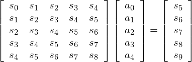
Where is the matrix containing our bit string, contains the coefficients of our LFSR, and contains more values of our bit string. Using the bit string we generated in the example above (1010100100), we will construct our matrices and solve for :

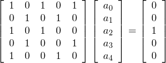
Now to solve, we just invert and solve for :

We can do all this in matlab using the following commands:

S = [1,0,1,0,1;0,1,0,1,0; 1,0,1,0,0; 0,1,0,0,1; 1,0,0,1,0];
S_gf = gf(S);       % tell matlab our matrix is in gf(2)
x = [0,0,1,0,0];
x_gf = gf(x);       % tell matlab our vector is in gf(2)
invS = inv(S)       % calculate the inverse of S in gf(2)
a = invS * x'

and the results:

inverse of S:
           1           1           1           1           1
           1           0           1           1           0
           1           1           0           1           1
           1           1           1           1           0
           1           0           1           0           0
a = 
           1           1           0           1           1

So we have recovered the vector of coefficients that we used for our example! One of the drawbacks with this algorithm, though, is that we needed to know L before we started. Often, L is something we want to know in addition to the coefficients. This is where the Berlekamp–Massey algorithm comes in, as it also determines L.

The Berlekamp–Massey Algorithm §

The Berlekamp–Massey (BM) Algorithm is an iterative algorithm that starts with the assumption that L=1, then tries to generate the given sequence using the putative LFSR. If it matches, we are done, otherwise it increases L and modifies the coefficients so there everything matches, then tries again.

comments powered by Disqus